Inside Outside Problem

A new month, a new DMCommunity challenge! In this month’s challenge, we are tasked with optimizing a production process:

Inside Outside Problem

You need to help a manufacturer decide how much of each demanded product should be produced internally and how much should be sourced from outside. Whether a product is made inside or outside, it has an associated cost. A product can consume a given amount of internal resources that have limited capacities. The general objective is to minimize the total production cost while ensuring the company meets the demand exactly or with a certain tolerance.

The manufacturer wants to consider various production decisions to choose the most suitable ones based on the long-term resource availability and uncertain future demand.

Here are examples of the data:

Seems like a fun optimization problem, which we can easily model in cDMN. However, the description also stresses that the manufacturer wants to consider multiple decisions. To meet this requirement, we will first model the problem as-is, and then we’ll add some additional options which allow a user to tweak the optimization.

Let’s begin with the cDMN glossary to declare the symbols of our problem domain. As per usual, we start with the types, i.e., domains of elements. In this case, this means declaring the various products and resources.

Type
Name	Type	Values
Product	string	P1, P2, P3
Resource	string	R1, R2, R3

Next, we’ll introduce our function symbols. These can be seen as a mapping from one or more types to another type. For instance, the first function (demand of Product) will map each Product on an Integer type. Similarly, we declare the costs of the product, the capacity of the resources, the number of resources required for each product, the number of product produced in-/outside, and finally, the total usage of each resource.

Function
Name	Type
demand of Product	Int
inside cost of Product	Int
outside cost of Product	Int
capacity of Resource	Int
nb Resource required for Product	Int
nb Product produced inside	Int
nb Product produced outside	Int
usage of Resource	Int

Finally, we finish off our glossary by introducing a constant which we’ll use to keep track of the total production costs (our minimization target).

Constant
Name	Type
total cost	Int

Now that all symbols are declared, we can (a) define those we already know using data tables, and (b) express rules and constraints over them. Let’s start with the first task, and declare our data tables.

Product data
D	Product	demand of Product	inside cost of Product	outside cost of Product
1	P1	250	6	8
2	P2	300	8	9
3	P3	200	3	4

Resource data
D	Resource	capacity of Resource
1	R1	1200
2	R2	800
3	R3	700

Resource data
D	Resource	Product	nb Resource required for Product
1	R1	P1	5
2	R2	P1	2
3	R3	P1	0
4	R1	P2	4
5	R2	P2	4
6	R3	P2	0
7	R1	P3	3
8	R2	P3	0
9	R3	P3	6

These tables define some product data (demand and costs), the demand of the resources, and the number of resources required to make a product. With our data tables finish, we can go into the rules and constraints.

The first one’s pretty simple: our total production (internal + external) should meet the total demand for each product. Here, we use a constraint table (E*) to ensure these values match. The table reads “For each product must hold that the demand of the product is equal to its number produced inside + its number produced outside”. (Note: the last two columns express that a product cannot have a non-negative production.)

Meet demand
E*	Product	demand of Product	nb Product produced inside	nb Product produced outside
1	-	nb Product produced inside + nb Product produced outside	≥ 0	≥ 0

Next, we should calculate the total cost. Again, pretty straightforward. In this case, we use a count (C+) table: “The total cost is calculated as the sum of each product’s internal production * internal cost plus external production * external cost”.

Calculate total cost
C+	Product	total cost
1	-	(nb Product produced insides * inside cost of Product) + (nb Product produced outside * outside cost of Product)

We calculate the usage of each resource in a similar manner, by multiplying the internal production by the required resources.

Calculate capacity
C+	Resource	Product	usage of Resource
1	-	-	nb Product produced inside * nb Resource required for Product

Using this total usage, we can now introduce a new constraint table (E*) to explicitly prevent exceeding the capacity of a resource.

Don't exceed capacity
E*	Resource	usage of Resource
1	-	≤ capacity of Resource

This already concludes our first model, in three data tables and four simple decision/constraint tables. :-) We can now have the cDMN solver optimize the cost, giving us the following result:

Model 1
==========
nb_Product_produced_inside := {P1 -> 240, P2 -> 0, P3 -> 0}.
nb_Product_produced_outside := {P1 -> 10, P2 -> 300, P3 -> 200}.
usage_of_Resource := {R1 -> 1200, R2 -> 480, R3 -> 0}.
total_cost := 5020.

Elapsed time: 0.035s

I.e., producing 240 of P1 internally and all the rest externally will give us an optimal cost of 5020. This is not really surprising, as P1 benefits the most cost-wise from inside production.

However, it does use up all of R1, and uses no R3. With possible “uncertain futures” in mind, fully using up an internal resource seems unwise. Similarly, fully relying on external production for P2 and P3 is likely not preferred either.

To fix this, let’s extend our model with the following:

A way to set the max% of resource usage
A minimal internal production percentage (i.e., at least 10% of each product should be produced internally)
A maximal external production percentage (i.e., at most 80% of each product may be produced externally)

First, we need to update our glossaries with some new symbols. In this case, we luckily only need to update our constants to add these new variables:

Constant
Name	Type
total cost	Int
capacity percentage margin	Real
max percent external	Real
min percent internal	Real

Our resource usage constraint now requires updating. Instead of blankly stating the usage may not exceed the capacity, we need to include the capacity percentage margin.

Don't exceed capacity
E*	Resource	usage of Resource
1	-	≤ capacity of Resource * (capacity percentage margin /100)

For the last modification, we add a new constraint table to state our min/max production constraints:

Extra product constraints
E*	Product	nb Product produced inside	nb Product produced outside
1	-	> (min percent internal/100) * demand of Product	< (max percent external/100) * demand of Product

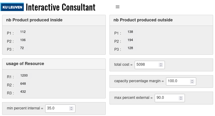
And that’s it! Using a new D-table, our production engineer can now set the values for these configuration variables, and find the best solution. Or, even better, they can use our interactive online environment to quickly try out different values and see the results. If you want to do so yourself, click on the link, and then click on “Interactive Consultant” at the top.

Playing around in this environment gives us the following three solutions for some input values of capacity and min/max in-/external:

Capacity Percentage	Max External	Max Internal	Optimal Cost
100	80	10	5065
80	80	10	5161
100	90	35	5098

The following screenshots show the full solutions in our online environment. (Note: input in white = user input, grey = derived by system after minimizing total cost)