cDMN Notation
The cDMN notation is based on the DMN standard, an open standard by the Object Management Group (who also specify the UML standard). If you already know standard DMN, learning cDMN shouldn’t be too hard. If you don’t know DMN, getting the hang of cDMN might take some practice. However, after modeling a few examples, you will be able to model your own cDMN problems before you know it.
1. cDMN vs DMN
cDMN adds four main features:
- constraint reasoning;
- quantification;
- more expressive data;
- data tables.
These additions are further explained in the following subsections.
2. Features
2.1 Constraint reasoning
By allowing to set constraints in the models, more complex problems can be modeled in a readable manner. Moreover, constraint tables are not forced to set a default value when no rule applies. Because of this, rather than define a single solution, a cDMN implementation defines a solution space.
2.2 Quantification
Quantification allows for creating more compact and maintainable tables. Instead of a row only applying for a specific element, it can now apply to every element part of a specific subset.
2.3 More expressive data types
Standard DMN variables are 0-ary functions (known as constants). They require no argument (thus 0-ary) and return a single value. cDMN adds three more data types:
- functions;
- relations;
- booleans.
These allow for a more flexible usage of knowledge and for a better design of tables.
2.4 Data tables
When modelling a problem in cDMN, we divide it in two parts:
- the problem logic;
- the actual problem instance, i.e. what specific problem to solve.
Example
For the map coloring problem, in which we want to color a map so that no two countries share the same color, we have the following division:
- Problem logic: color a map so that no two countries share a color;
- Problem instance: the specific map to color.
In cDMN, the problem instances are represented via data tables. This allows for the application of a single cDMN model to multiple problems, by simply switching out the data tables.
3. Tables
3.1 Glossary
Before writing any business logic, rules or constraints, a specific set of terms need to be defined. We use multiple glossaries for this purpose, with each glossary a list of specific kinds of terms. In total there are five different glossaries:
| Table | Explanation | Relevant Columns |
|---|---|---|
| Type | A type can be seen as a domain of possible elements. | Name, Type, Values |
| Function | Functions map an amount of types on a single type. | Name, Type |
| Constant | A constant maps a name on a single type. | Name, Type |
| Relation | Relations specify a connection between types. | Name |
| Boolean | Booleans map a type on either True, or False. | Name |
More explanation of the five different glossaries can be found in the rest of the section, including examples.
3.1.1 Types
A type can be seen as a definition of a domain of possible elements.
For example, all integer numbers can be grouped as one type.
Or, all the people working at a company could be grouped as the type Employees.
cDMN knows 4 basic types, which can be used in the glossary without needing explicit definitions. All other types need to be derived from these basic four types (subtyping).
| Type | Explanation |
|---|---|
| Int | An integer number, ranging from -∞ to +∞. |
| Real | A number containing a comma, ranging from -∞ to +∞. |
| String | Normal text. |
| Datestring | A representation for dates, in the OSI 8601 format. (this is currently experimental) |
These basic types are used to create subtypes. This allows a more readable notation, and a reduction of possible values of a type.
For instance, in the following snippet the type glossary of the Reindeer_Ordering challenge is shown.
Here, we define 3 types: Reindeer, Place and Relative.
| Type | ||
|---|---|---|
| Name | Type | Values |
| Reindeer | string | Comet, Rudolph, Prancer, Cupid, Donder, Vixen, Dancer, Dasher |
| Place | int | [1,9] |
| Relative | string | inFront, Behind |
Subtyping has 2 main advantages:
- The name of the type is easier to interpret (
stringvsReindeer)- It’s possible to set a more narrow set of possible values of a type.
A string in itself could be anything: e.g. it could be a, b, procrastination, yes, etc.
By subtyping string into the type Reindeer, we can narrow down the possible types to just the names of the reindeer.
The same is done for Place, which is a subtype of integers.
Subtyping here allows us to set a range of integers, which makes sure that there can never be a Place outside of the range [1,9].
In the Name column, we write the name of our type.
This name can be any string, but should be something descriptive of the type it’s specifying.
In the Type column, we can refer to the supertype we’d like to use.
This can be one of the 4 basic types, or another type that is already declared in the glossary.
In the last column, Values, we can write down all the elements that are containing in our type.
For instance, for the type Reindeer, these are the names of all the reindeer.
For Place, we define a range of integers, from one to nine.
Thus, our range is defined as the following values: 1, 2, 3, 4, 5, 6, 7, 8, 9.
A well-defined range can make the difference between a short and a long solving time.
Note
For string, the column values can be left undefined by inserting a - or by referring to a data table containing those values.
In both cases, there should be a data table defining the string. See 3.4 Data tables.
Important
Subtypes of floats and integers should always have a defined range.
3.1.2 Functions
A function in cDMN is a mapping of arguments on a single type. This is especially useful when there’s a functional link between two sets of elements. For example, a set of people can be easily mapped on a set of dates of birth using a function. Every person has exactly one date of birth, but a date of birth can have multiple people being born on it.
Note
The term “function” in cDMN is not be confused with “function” in programming. cDMN uses the mathematical meaning.
In the Name column, we write down the name for our function.
However, this name can not just be anything: there is a specific syntax for functions.
The syntax is fairly straightforward: it can be any name as long as the argument types are clearly part of it.
For example, value of Argument is a function to map an instance of Argument on something else.
It’s possible to list multiple arguments, each of which should be a known type.
For instance, in the Reindeer problem our Function glossary could look as follows.
| Function | |
|---|---|
| Name | Type |
| order of Reindeer | Place |
| Partial relativeposition of Reindeer and Reindeer | Relative |
The function order of Reindeer will assign a value of the type Place to each Reindeer.
It makes sense to use a function for this purpose, as each reindeer needs a position, and can only have a maximum of one position.
There is a direct connection between the two types.
Note
It’s currently impossible to use int as a super type for a function, because it doesn’t have a set range of values. You should always define a subtype of integers, and assign it a correct range.
Warning
Make sure that there are no other types in the name other than the argument types, or the solver will add them to the list of arguments. For example, place of Reindeer represents a function with two arguments, namely Place and Reindeer.
In order to only have the Reindeer argument, write the Place with a lowercase: place of Reindeer.
Partial Function
A partial function acts like a normal function, except that not every argument needs to map to a value. Hence the name partial function.
Warning
Take extreme caution when using a partial function. When quantifying over a partial function, make sure you only use the arguments for which a value is set in the partial function.
Constant
The constant is a special type of function, where no argument is used.
It only contains one value, instead of a value for each type of argument.
This can e.g. be used when defining a cost for a problem, as demonstrated in the following glossary snippet.
Note how the keyword of isn’t used.
| Constant | |
|---|---|
| Name | Type |
| Total Sodium | Nat |
| Total Fat | Nat |
| Total Calories | Nat |
| Total Cost | Nat |
3.1.3 Relations
A relation can be seen as a function and produces either Yes or No.
Unlike the function, the relation has no specific syntax. Any string can form a relation, as long as it contains type names. There can be as many types listed as needed, in every possible order with any possible word in between.
For example, in the Map_Coloring challenge, the glossary is as follows.
| Relation |
|---|
| Name |
| Country border Country |
Boolean
A special type of relation is the boolean. It’s a relation which doesn’t have any arguments, and it can only be true or false.
3.2 Decision tables
The decision table is the bread and butter of DMN/cDMN. It allows the user to model a basic decision, in the form of a simple table. An example of an annotated decision table can be found below.
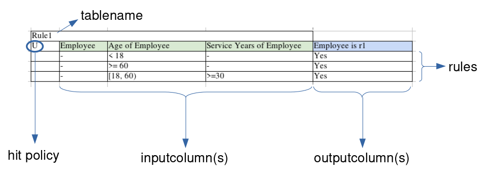
The table decides for every employee whether or not they are eligible for extra vacation days. The text it models is listed in the following example.
Example: vacation days eligibility
All employees under 18 years or over 60 get 5 extra vacation days (they apply for rule1). If an employee is between those ages, but has more or equal to 30 service years, they also get the extra days.
This example is implemented as three rows in the decision table.
It checks for every employee (the - translates to a don't-care, thus for every employee), every age of employee and every number of service years of employee whether or not they’re eligible for the vacation days.
A translation of the table rules to English would be as follows:
- Every employee, younger than 18, with any amount of service years is eligible.
- Every employee, older or equal to 60, with any amount of service years is eligible.
- Every employee, between age 18 (included) and 60 (excluded) with more or equal to 30 years of service years is eligible.
Note
If for a specific employee none of the rules are satisfied, the relation Employee is r1 is automatically considered as untrue. There is no seperate rule needed to define this.
This specific decision table has the Unique hitpolicy, denoted by the U in the top-left corner of the table.
This means that at most only 1 row can be satisfied, and there is no overlap between the rows.
For a table of other hitpolicies, see 3.2.1 Hitpolicies.
Note
A decision table can have any amount of inputs (even zero), and needs at least one outputcolumn.
3.2.1 Hitpolicies
| Decision hitpolicy | Explanation |
|---|---|
| U | Unique: only one rule can be satisfied. |
| A | Any: any of the rules can be satisfied. |
| F | First: only the first rule eligible is satisfied. |
| C+ | Sum: sum the values of each satisfied row. |
| C< | Minimum: take the minimum value of each satisfied row. |
| C> | Maximum: take the maximum value of each satisfied row. |
| C# | Count: count the amount of satisfied rows. |
For more examples on these hitpolicies, see the Examples.
3.2.2 Using the same type twice
In cDMN it’s possible to use the same type as many times as you like in a single table.
To differentiate between multiple instances of the same type, the syntax Type called typename is introduced.
The following table shows an example.
| Match | |||||
|---|---|---|---|---|---|
| U | Person called p1 | Person called p2 | p1 Likes p2 | p2 Likes p1 | p1 Matches p2 |
| 1 | - | not(p1) | Yes | Yes | Yes |
In text, this table reads as: “For every Person p1 and Person p2, if p1 likes p2 and p2 likes p1, then p1 matches p2.”
Note
Note how we have to explicitly define that p1 does not equal p2.
3.2.3 Syntax in cells
Inside a decision table cell, only a certain syntax is allowed. The below table shows every possible syntax that a cell can have.
| Cell | Explanation |
|---|---|
| - | don’t care: the rule goes for every possible value of the inputcolumn. |
| Yes/No | Can be used when trying to specify the status of a specific relation. |
| not(type) | (function): Specifies that it can’t be the same value. |
| not(relation) | returns the inverted value of the relation. |
| val | usefull when you want a rule to only count for one specific value of a type. |
| <= x; >= x; < x; > x; = x | Used to compare two values. |
| [x,y] | inclusive range, the value needs to be between x and y or equal to x or y. |
| (x, y] | the value needs to be between x and y, or equal to y. |
| [x, y) | the value needs to be between x and y, or equal to x. |
| (x, y) | the value needs to be between x and y. |
| #Type | the number of elements in type Type. |
3.3 Constraint tables
A constraint table is used when a list of constraints needs to be modeled.
It can be seen as a decision table in which each row needs to be satisfied.
It is denoted by the “Every” hit policy, as in “every rule needs to be satisfied”.
In tables, it is denoted by E*.
| Bordering countries can't share colors | ||||
|---|---|---|---|---|
| E* | Country called c1 | Country called c2 | c1 Borders c2 | Color of c1 |
| 1 | - | - | Yes | not(Color of c2) |
For instance, in the Map Coloring problem, we want to define that if two countries share a border, they should have a different color. In text, this is written as “For every country c1, country c2 holds that if c1 and c2 share a border, the color of c1 cannot equal the color of c2”.
It’s also possible to define multiple constraints, where each one needs to be satisfied. This is shown in the Monkey Business example.
| Monkey Constraints | |||||
|---|---|---|---|---|---|
| E* | Monkey | place of Monkey | fruit of Monkey | place of Monkey | fruit of Monkey |
| 1 | Sam | - | - | Grass | not(Banana) |
| 2 | - | Rock | - | - | Apple |
| 3 | - | - | Pear | not(Branch) | - |
| 4 | Anna | - | - | Stream | not(Pear) |
| 5 | Harriet | - | - | not(Branch) | - |
| 6 | Mike | - | - | - | not(Orange) |
This table translates into the following rules:
- For each monkey, if the monkey is named Sam, then the place of the monkey is Grass and the fruit is not Banana.
- For each monkey, if its location is Rock, then the fruit of the monkey is Apple.
- For each monkey, if its fruit is Pear, the place of the monkey is not the Branch.
- For each monkey, if the monkey is named Anna, its place is the Stream and it’s fruit is not the Pear.
- For each monkey, if the monkey is named Harriet, its place is not the Branch.
- for each monkey, if the monkey is named Mike, then its fruit is the Orange.
3.4 Data tables
The data table allows the user to input data that doesn’t really fit in a decision table.
Although technically you could use the Unique hitpolicy to input data, a data table will always work faster.
Another advantage is that not every instance of a type needs to be listed in the values column of the glossary.
Note
If any of the decision tables or constraint tables holds a specific type value (for instance, the name of the monkeys in the previous table) you still need to explicitly list those values in the glossary.
A simple example of a data table is the one found in Hamburger Challenge. Per ingredient, we input its sodium, fat and calories amount and the cost.
| Data Table: Nutritions | |||||
|---|---|---|---|---|---|
| Item | sodium of Item | fat of Item | calories of item | cost of Item | |
| 1 | Beef Patty | 50 | 17 | 220 | 25 |
| 2 | Bun | 330 | 9 | 260 | 15 |
| 3 | Cheese | 310 | 6 | 70 | 10 |
| 4 | Onions | 1 | 2 | 10 | 9 |
| 5 | Pickles | 260 | 0 | 5 | 3 |
| 6 | Lettuce | 3 | 0 | 4 | 4 |
| 7 | Ketchup | 160 | 0 | 20 | 2 |
| 8 | Tomato | 3 | 0 | 9 | 4 |
A data table can also do most of the things that works in a normal decision table/constraint table. For instance, it can also quantify over the same type multiple times.
| Data Table: bordering countries | |||
|---|---|---|---|
| Country called c1 | Country called c2 | c1 Borders c2 | |
| 1 | Belgium | France, Luxembourg, Netherlands, Germany | Yes |
| 2 | Netherlands | Germany | Yes |
| 3 | Germany | France, Denmark, Luxembourg | Yes |
| 4 | France | Luxembourg | Yes |
As mentioned earlier, a data table also allows us to leave the Values column empty for a type in a data table.
This is especially useful when we have a lot of data.
For example, in the Balanced Assignment challenge we have a list of 210 people.
Each person has a name, department, location, gender and title.
Without a data table, each of these types needs to be listed in the Values column.
Instead of having to type all this data, we can just copy-paste the employee list into a data table!
Caution
When using data tables to set the values of a function, you should make sure that it is complete. In other words, every possible set of inputs for the function should have a defined output.
4. Goal
In standard DMN, there is always only one solution possible for every set of inputs.
In cDMN however, we do not define a single solution but rather a solution space.
To specify which specific solution we want from this space, the Goal table is used.
At the moment, there’s four possible goals allowed in a cDMN model.
| Inference | Explanation |
|---|---|
| Get {x} models | This will find x amount of solutions. |
| Minimize {val} | This will find the solution with the lowest value for val. |
| Maximize {val} | This will find the solution with the highest value for val. |
| Propagate | This will derive the consequences of the model. I.e., those values that are always true, or always false. |
An inference method can be specified using an Goal table.
Some examples are given below.
Note
If no Goal table is specified, cDMN will default to finding one model.
| Goal |
|---|
| Get 10 models |
| Goal |
|---|
| Minimize TotalPrice |
| Goal |
|---|
| Maximize Score |
A.1: Annotations
cDMN decision and constraint tables support an optional column Annotations, which can e.g. be used to explain where a rule comes from or what its natural language meaning is. These annotations are not interpreted by the cDMN solver, and are meant purely for human readers. The table below shows an example of annotations being used in the Monkey Problem:
| Monkey Constraints | ||||||
|---|---|---|---|---|---|---|
| E* | Monkey | place of Monkey | fruit of Monkey | place of Monkey | fruit of Monkey | Annotation |
| 1 | Sam | - | - | Grass | not(Banana) | Sam on grass without banana |
| 2 | - | Rock | - | - | Apple | Monkey on rock ate apple |
| 3 | - | - | Pear | not(Branch) | - | Pear eater not on branch |
| 4 | Anna | - | - | Stream | not(Pear) | Anne in stream without pear |
| 5 | Harriet | - | - | not(Branch) | - | Harriet not on branch |
| 6 | Mike | - | - | - | not(Orange) | Mike didn't eat orange |